Quick Start:
Instructions, technical details, and other information is available through the
eRAMS resource center.
- Create a river cross-section:
- Select "Create on Map" to extract a cross-section from a DEM:
- Zoom to the stream/river channel of interest
- Click "Create"
- Single-click a start point on the map
- Single-click an end point on the map, this defines a transect within the channel
- Select "Create from Spreadsheet" to create a cross-section from an uploaded spreadsheet:
- Click "Create"
- Specify Start and End point Latitudes and Longitudes
- Latitude and Longitude for a location can be extracted from the map by clicking From Map
- Click "Upload Spreadsheet" to select a csv file to upload. This information will then be used to create a cross-section
- Select and Use/Edit a cross-section:
-
Once a cross-section is selected, the
 icon represents the x=0 location for the selected cross-section
- Click "View" to launch the edit/view interface for the selected cross-section
- Click "Delete" to permanently delete the selected cross-section
- Further Questions:
- For questions about how each part of the cross-section tool works select the "Further Info." button on the bottom of the interface
- For more detailed instructions about inputs click the "Help" button on the bottom of the interface
From Spreadsheet:
The specified latitude and longitude for the end point does not need to line up exactly with the last point in the spreadsheet, the tool will adjust the length of the cross-section's line on the map as needed.
- You can also use the "From Map" buttons to extract the latitude and longitude of a point selected from the map rather than typing in your cross-section's latitude and longitude.
File Format Instructions:
To work with this analysis tool the uploaded file must be a two-column, comma separated value (CSV) file.
- The first row must contain a label for the columns like "x, y".
- The remaining rows must contain pairs of x-y points of a cross-section with the first row containing x = 0 (column 1) and its associated elevation (column 2).
- The units of x and y should be meters.
USGS National Elevation Dataset (NED):
In addition to being able to use uploaded rasters of elevation data, eRAMS access the
National Elevation Dataset
(NED). Each cross-section point that is calculated accesses this dataset through the
NED Point Query Service
which calculates the elevation of a point based on its latitude and longitude.
Editing a Cross-Section Help:
-
The
 icon allows a new point, station (x) and elevation (y) to be added to the cross-section.
-
The
 icon allows the current point, station (x) and elevation (y), to be removed from the cross-section.
- Each point's station (x) and elevation (y) is editable, once you have made a change and hit enter or click off of the box you edited and the graph will update to view the changes.
- Clicking Append Spreadsheet will allow you to upload a spreadsheet with the below properties and add it to the existing cross-section as more points. See below for file format instructions.
- Clicking Download Cross-Section download a csv file with the start and end latitudes and longitudes as well as all the cross-section locations (x) and elevations (y).
- Clicking Save Changes will permanently save the modified version of the cross-section.
- Clicking Reset will restore the cross-section to its original un-edited version.
File Format Instructions:
To work with this analysis tool the uploaded file must be a two-column, comma separated value (CSV) file.
- The first row must contain a label for the columns like "station (x), elevation (y)".
- The remaining rows must contain pairs of station (x) and elevation (y) points of a cross-section with the first row containing station x = 0 (column 1) and its associated elevation (column 2).
- The units of station (x) and elevation (y) should be meters.
Interface Buttons:
- Clicking Further Info. open details about cross-section points and editing.
- Clicking Help will bring up this window.
- Clicking Download will download a csv file containing the cross-section points, station (x) and elevation (y), as well as the start and end latitude/longitude points.
- Clicking Calculate is not available on this tab.
Hydraulic Properties Help:
- Specify a depth of flow using one of the following methods:
- User-Defined Flow Depth
- If you know the depth of flow you are interested in, use this choice.
- Critical Depth
- If you know flow conditions cause a critical depth of flow to occur here, specify the discharge in the channel to calculate and use the critical depth at this cross-section.
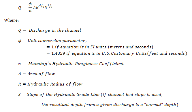
- Normal Depth (Manning's Equation)
- If you know flow conditions cause a normal depth of flow to occur here; specify the following and a normal depth will be calculated using Manning's Equation (1891):
- Discharge in the channel
- Channel bed slope
- Manning's Hydraulic Roughness Coefficient, n
- Click Calculate to determine the cross-section hydraulic properties based on the flow depth, further info. about these is available here.
Cross-Section Sediment Transport
- Select a Sediment Transport Equation
- Click here or see "Further Info." after calculation of hydraulic properties for more details on the sediment transport equations.
- Specify the required inputs
- Click Calculate to calculate sediment transport through the cross-section
Interface Buttons:
- Clicking Further Info. open details about how to determine a depth of flow for cross-section properties or information about sediment transport relationships if the user has already calculated the cross-section's hydraulic properties.
- Clicking Help will bring up this window.
- Clicking Download will download a csv file containing the cross-section points, station (x) and elevation (y), as well as the start and end latitude/longitude points.
- Clicking Calculate will calculate cross-section hydraulic properties or sediment transport if the user has already calculated the cross-section's hydraulic properties.
Sediment Yield Help:
- Specify a Flow Duration Curve:
- Gauge Station Data
- Search for a near by stream gauging station and use it's flow record to create a flow duration curve of exceedance values for each flow.
- Uploaded Data
- Upload a csv file of your own flow duration curve for the cross-section's flows.
- To work with this analysis tool the uploaded file must be a two-column, comma separated value (CSV) file.
- The first row must contain a label for the columns "flow duration curve, flow (cfs)".
- The remaining rows must contain pairs of flow exceedances (column 1) and their associated flows (column 2).
- The units of exceedance are on a percent scale from 0 (the largest flow) to 100 (the lowest flow) and flows should be in cubic feet per second (cfs).
- Select a Sediment Transport Relationship (see further info. for more details):
- Specify the required inputs.
- Click Calculate to use the sediment transport relationship in the calculation of an effective discharge and a half-load discharge.
- Additional information about the sediment equations can be found here.
Interface Buttons:
- Clicking Further Info. open details about what an effective discharge and a half-load discharge are as well as details about the inputs required to determine them.
- Clicking Help will bring up this window.
- Clicking Download will download a csv file containing the cross-section points, station (x) and elevation (y), as well as the start and end latitude/longitude points.
- Clicking Calculate will calculate the effective discharge, half-load discharge, and cumulative sediment yield curve for the current cross-section, flow duration curve, and sediment transport.
Manning's Hydraulic Roughness Coefficient, n Help:
One variable required by Manning's Equation for calculation of a 'normal' depth is a hydraulic roughness coefficient, n. This coefficient takes into account roughness from submerged channel bed forms, vegetation, and more. 'Normal' depth of flow in a channel is very sensitive to the value of n and changes with depth as various roughness-factors (vegetation, boulders, etc.) become submerged or revealed. While there is great variability in the roughness parameter, n, some simplified guidance is provided below based on a number of different studies.
Variation of Manning's Roughness Coefficient, n, with Channel Bed Type (adapted from Shen et al., 2003, Table 12.2.1)
| Bed Characteristics |
Reference Manning's Roughness Coefficient, n |
| Sand: |
|
| - Plane Bed: |
0.011 - 0.020 |
| - Ripple Bed: |
0.018 - 0.035 |
| - Dune Bed: |
0.020 - 0.035 |
| - Standing Waves: |
0.014 - 0.025 |
| - Antidunes: |
0.015 - 0.035 |
| Gravel and Cobbles: |
0.020 - 0.030 |
| Boulder: |
Roughness varies greatly. Usually roughness increases with decreasing flow depth. n can reach 0.1 |
| Vegetation: |
Roughness varies greatly with changes of density, height, flexibility of vegetation, and the relative ratio between flow depth and vegetative elements |
| Bermuda, Kentucky, Buffalow Grasses: |
Flow depth more than 5 times vegetation height: n between 0.01 and 0.2 |
| Extremely Dense Vegetation: |
Vegetation height above flow depth: n can exceed 1 |
| Natural Sandy Streams: |
|
| - Clean and Straight: |
0.025 - 0.04 |
| - Winding and Some Weeds: |
0.03 - 0.05 |
| Mountain Streams with Boulders: |
0.04 - 0.1 |
| Floodplains: |
|
| - Short Grass: |
0.02 - 0.04 |
| - High Grass: |
0.03 - 0.05 |
| - Dense Willow, Brush, etc.: |
0.05 - 0.20 |
References:
Shen, Hsieh Wen, and Pierre Y. Julien. 1993. "Chapter 12: Erosion and Sediment Transport." The McGraw Hill Handbook of Hydrology. D. R. Maidment, ed., McGraw-Hill New York
Disclaimer:
These outlines, the tables, and the graphs are not intended for final designs, but instead are intended to inform preliminary thinking on hydraulics and guide future analyses. The developers are not liable for use of this model (including but not limited to information extracted and results).
Channel Sediment Size Help:
While there is great variability in the sediment sizes in river channels, some simplified guidance is provided below:
Sediment Grade and Sizes (adapted from Wentworth, 1922; Table I)
| Sediment Name |
Size [mm] |
| - Boulder: |
> 256 |
| - Cobble: |
64 - 256 |
| - Pebble: |
4 - 64 |
| - Granule: |
2 - 4 |
| - Very Coarse Sand: |
1 - 2 |
| - Coarse Sand: |
0.5 - 1 |
| - Medium Sand: |
0.25 - 0.5 |
| - Fine Sand: |
0.125 - 0.25 |
| - Very Fine Sand: |
0.0625 - 0.125 |
| - Silt: |
0.004 - 0.0625 |
| - Clay: |
< 0.04 |
References:
Wentworth, C.S. 1922. "Scale of Grade and class Terms for Clastic Sediments." The Journal of Geology, Vol. 30(5): 377-392
Disclaimer:
These outlines, the tables, and the graphs are not intended for final designs, but instead are intended to inform preliminary thinking on hydraulics and guide future analyses. The developers are not liable for use of this model (including but not limited to information extracted and results).
Sediment Transport Equation Help:
Total Load Equations
Total load equations are typically used on fine grain sand bed rivers because they calculate the total sediment transported in the water column. The equations in this interface which are total load equations for fine grain and sand bed rivers are:
- Yang's Sand Total Load Equation (1996)
- Brownlie's Total Load Equation (1981)
- Power-Function Rating Curve (derived from a separate analysis)
Bed-Load Equations
Bed-Load equations are typically used on coarse grain rivers like gravel bed and cobble rivers. The equations in this interface which are bed-load equations for gravel and cobble bed rivers are:
- Martin and Church's Revisitation of Bagnold's Bed Load Equation (2000)
- Wilcock and Kenworthy's Two-Phase Bed Load Equation (2002)
- Power-Function Rating Curve (derived from a separate analysis)
Further information about the details of the inputs for each sediment equation can be found here.
Cross-Section Tool Further Information:
Instructions, technical details, and other information available through the
eRAMS resource center.
- The
icon represents the x=0 location for a selected cross-section.
USGS National Elevation Dataset (NED):
In addition to being able to use uploaded rasters of elevation data, eRAMS access the 10-meter
National Elevation Dataset
(NED). Each cross-section point that is calculated accesses this dataset through the
NED Point Query Service
which calculates the elevation of a point based on its latitude and longitude.
Cross-Section Points:
A cross-section is created by starting from the provided start point (Latitude and Longitude) and moving towards the end point (Latitude and Longitude) at a given spacing.
- If the eRAMS elevation dataset is used, the spacing is set to 10 meters which is the raster cell size of the elevation dataset.
- If an uploaded elevation raster is used, the spacing is set equal to the cell size of the uploaded raster.
- If using both the eRAMS elevation dataset and an uploaded elevation layer (like lidar data) the spacing is initially set to 10 meters from the start point. Then after moving 10 meters along the line between the start and end points, the algorithm checks if the new point on the line is within the uploaded raster or not. If it is within the raster, it changes the spacing to the raster's cell size and continues towards the end point. If the point is not in the raster it continues using the 10 meter spacing.
Cross-Section Hydraulic Properties:
Instructions, technical details, and other information available through the
eRAMS resource center.
Once a cross-section has been created, the user has the ability to calculate its hydraulic properties, namely area, wetted-perimeter, top-width, hydraulic-radius, hydraulic-depth. However, in order to calculate these properties a flow depth is required. There are numerous ways to enter a flow depth for use with this tool:
- User-Defined Flow Depth
- If you know the depth of flow you are interested in, use this choice.
- Critical Depth
- If you know flow conditions cause a critical depth of flow to occur here, specify the discharge in the channel to calculate and use the critical depth at this cross-section.
- Normal Depth (Manning's Equation, 1891)
- If you know flow conditions cause a normal depth of flow to occur here; specify the following and a normal depth will be calculated using Manning's Equation (1891) based on the provided channel roughness:
Manning's Equation:
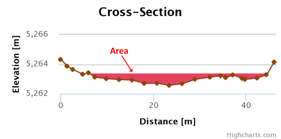
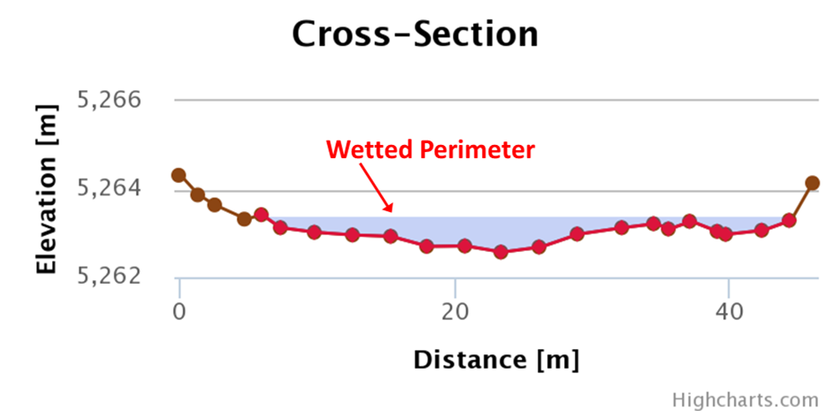
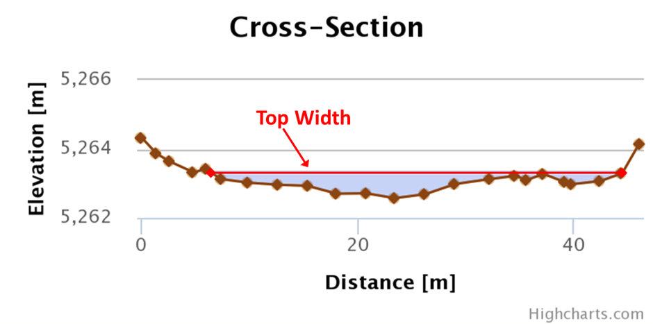
One assumption of the calculations for channel properties is: if the depth of water is higher than the left and/or right edge point(s) of the cross-section, a vertical edge wall is assumed at that edge. For this reason it is recommended to make sure each cross-section not only includes points in the river but well out onto the floodplain as well. Each of these properties is shown below to better understand what they represent:
Area:
Wetted-Perimeter:
Top-Width:
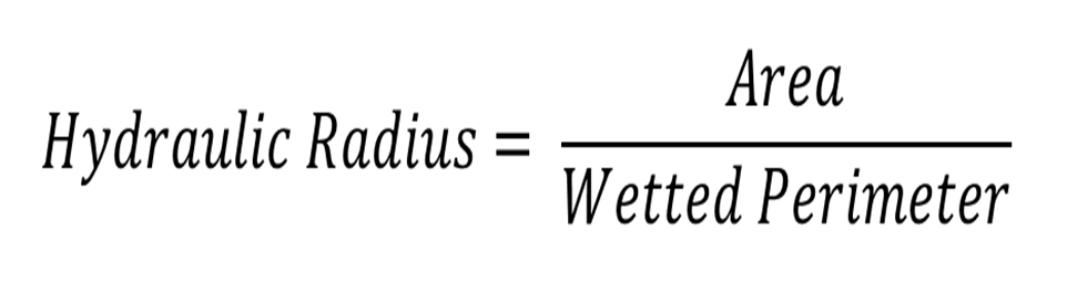
Hydraulic Radius:
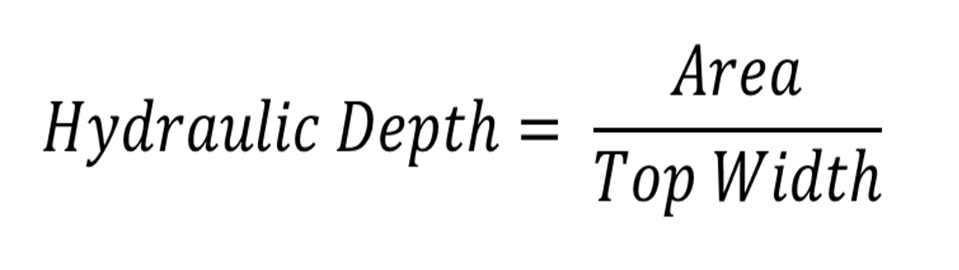
Hydraulic Depth:
References:
Manning, R. 1891. "On the flow of water in open channels and pipes." Transactions of the Institution of Civil Engineers of Ireland 20:161-207.
Disclaimer:
These outlines, the tables, and the graphs are not intended for final designs, but instead are intended to inform preliminary thinking on hydraulics and guide future analyses. The developers are not liable for use of this model (including but not limited to information extracted and results).
Sediment Transport:
Instructions, technical details, and other information available through the
eRAMS resource center.
A number of sediment transport equations are available in this tool. The equations and details for each are listed below:
Yang's Sand Total Load Equation (1996)
One choice for sediment transport is Yang's (1996) sand total load sediment transport equation. The sediment transport equation and parameter descriptions are shown below.
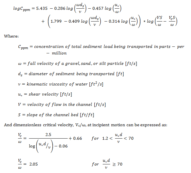
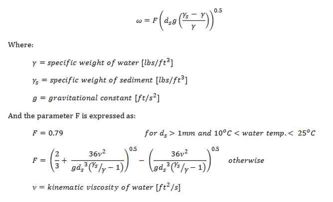
One important assumption of in the sediment transport calculated using Yang 1996 is that the fall velocity of the sediment particle is calculated using Rubey's Formula (1933), shown below:
Rubey's Formula for Fall Velocity (1933)
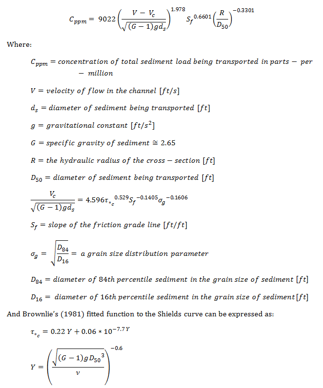
Brownlie's Total Load Equation (1981)
Another choice for a total sediment load calculation is Brownlie's 1981 equation for sediment transport as shown below.
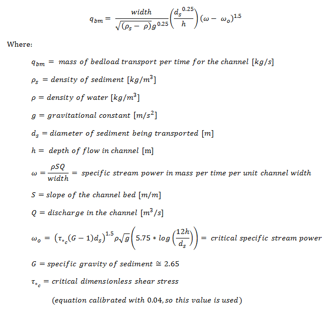
Martin and Church's Revisitation of Bagnold's Bed Load Equation (2000)
A further choice of sediment transport is the bed load equation originally developed by Bagnold (1980) as revisited and modified by Martin and Church (2000) as shown below:
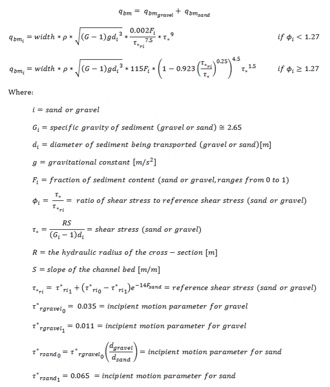
Wilcock and Kenworthy's Two-Phase Bed Load Equation (2002)
A further choice of sediment transport is the two-part (sand and gravel) bed load equation developed by Wilcock and Kenworthy (2002) for mixtures of sand and gravel as shown below:
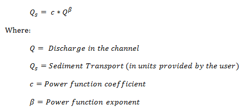
Power-Function Rating Curve
A cross-section independed choice of sediment transport is a power-function sediment rating curve. This is typically accomplished through a regression on existing gauge data for a stream gauging site to determine the coefficient and exponent of the relationship shown below:
References:
Brownlie, William R. 1981. "Compilation of Alluvial Channel Data: Laboratory and Field." W.M. Keck Laboratory of Hydraulic and Water Resources, Division of Engineering and Applied Science, California Institude of Technology, Pasadena, California. Report KH-R-43B.
Bagnold, RA. 1980. "An Emperical Correlation of Bedload Transport Rates in Flumes and Natural Rivers." Royal Society of London Proceedings A372:453-473.
Martin, Yvonne, Michael Church. 2000. "Re-Examination of Bagnold's Empirical Bedload Formulae." Earth Surface Processes and Landforms 25:1011-1024.
Rubey, W.W. 1933. "Equilibrium-Conditions in Debris-Laden Streams" Transactions, American Geophysical Union 14.
Wilcock, Peter R., Stephen T. Kenworthy. 2002. "A Two-Fraction Model for the Transport of Sand/Gravel Mixtures." Water Resources Research 38(10),1194.
Yang, Chih T., Albert Molinas, Baosheng Wu. 1996. "Sediment Transport in the Yellow River" Journal of Hydraulic Engineering 122:237-244.
Disclaimer:
These outlines, the tables, and the graphs are not intended for final designs, but instead are intended to inform preliminary thinking on hydraulics and guide future analyses. The developers are not liable for use of this model (including but not limited to information extracted and results).
Sediment Yield:
Instructions, technical details, and other information available through the
eRAMS resource center.
Effective Discharge:
The concept of an 'effective discharge' of a river was introduced by Wolman and Miller (1960) as the stream dischage that transports the most sediment over time. This is based on the argument that over long periods of time, small frequent flows will carry a greater amount of sediment than infrequent large flows. The effectiveness of a river's discharge is determined by multiplying the frequency of flows, probability density function (pdf), with the amount of sediment transported during each flow. The peak of this curve is called the 'effective discharge' although this must be interpreted carefully if the curve is not well defined or has more than one prominent peak.
Half-Load Discharge:
Due to variation in the interpretations and method of calculation of an 'effective discharge', there have been proposals to use new discharge indicies to represent sediment transport for stream flows. One such index is the 'half-load discharge' (Klonsky and Vogel; 2011) which is defined as the discharge above and below which half of the total sediment load is transported. Generally, the half-load discharge corresponds to a larger discharge than the effective discharge.
Flow, Cross-Section Hydraulics, and Sediment Transport:
Both the calculation of an effective discharge and a half-load discharge require an estimate of sediment transport at each flow as well as hydraulic properties like cross-sectional area and hydraulic radius. Rather than calculate this for each flow on record, a number of points (default 50, but can be changed under advanced options) are interpolated from the flow record. This interpolation may be linear or log interpolated between the maximum and minimum flows based on the users's selection under advanced options.
Then for each interpolated flow, a normal depth is assumed based on the cross-section and hydraulic roughness and other necessary hydraulic properties for the specified sediment transport relationship are calculated. A histogram of these bin-ned flows (based on the limits of the interpolated points) is also provided as output.
A number of sediment transport options are available in this tool and the equations and details for each are listed below:
Yang's Sand Total Load Equation (1996)
One choice for sediment transport is Yang's (1996) sand total load sediment transport equation. The sediment transport equation and parameter descriptions are shown below.
One important assumption of in the sediment transport calculated using Yang 1996 is that the fall velocity of the sediment particle is calculated using Rubey's Formula (1933), shown below:
Rubey's Formula for Fall Velocity (1933)
Brownlie's Total Load Equation (1981)
Another choice for a total sediment load calculation is Brownlie's 1981 equation for sediment transport as shown below.
Martin and Church's Revisitation of Bagnold's Bed Load Equation (2000)
A further choice of sediment transport is the bed load equation originally developed by Bagnold (1980) as revisited and modified by Martin and Church (2000) as shown below:
Wilcock and Kenworthy's Two-Phase Bed Load Equation (2002)
A further choice of sediment transport is the two-part (sand and gravel) bed load equation developed by Wilcock and Kenworthy (2002) for mixtures of sand and gravel as shown below:
Power-Function Rating Curve
A cross-section independed choice of sediment transport is a power-function sediment rating curve. This is typically accomplished through a regression on existing gauge data for a stream gauging site to determine the coefficient and exponent of the relationship shown below:
References:
Brownlie, William R. 1981. "Compilation of Alluvial Channel Data: Laboratory and Field." W.M. Keck Laboratory of Hydraulic and Water Resources, Division of Engineering and Applied Science, California Institude of Technology, Pasadena, California. Report KH-R-43B.
Bagnold, RA. 1980. "An Emperical Correlation of Bedload Transport Rates in Flumes and Natural Rivers." Royal Society of London Proceedings A372:453-473.
Klonsky, L., R.M. Vogel. "Effective Measures of 'Effective Discharge'." Journal of Geology 119:1-14.
Martin, Yvonne, Michael Church. 2000. "Re-Examination of Bagnold's Empirical Bedload Formulae." Earth Surface Processes and Landforms 25:1011-1024.
Rubey, W.W. 1933. "Equilibrium-Conditions in Debris-Laden Streams" Transactions, American Geophysical Union 14.
Wilcock, Peter R., Stephen T. Kenworthy. 2002. "A Two-Fraction Model for the Transport of Sand/Gravel Mixtures." Water Resources Research 38(10),1194.
Wolman, M.G., J.P. Miller. 1960. "Magnitude and Frequency of Forces in Geomorphic Processes." Journal of Geology 68:54-74.
Yang, Chih T., Albert Molinas, Baosheng Wu. 1996. "Sediment Transport in the Yellow River" Journal of Hydraulic Engineering 122:237-244.
Disclaimer:
These outlines, the tables, and the graphs are not intended for final designs, but instead are intended to inform preliminary thinking on hydraulics and guide future analyses. The developers are not liable for use of this model (including but not limited to information extracted and results).
Regional Flow Duration Curve:
A regional flow duration curve (FDC) is an averaging of multiple FDCs from a number of gauges in a particular geographic region which exhibits similar traits (climate, geology, etc.). There are a number of ways to regionalize a flow duration curve given gauge data (statistical regression, parametric fitting, or graphical methods (Castellarin et al., 2004)). The method used here is a graphical method similar to that used by Smakhtin et al. (2000) in which each individual gauge's flow duration curve is normalized based on a metric like drainage area, long-term averge flow, or another flow metric like Q2 or bankfull discharge. These normalized flow duration curves are then averaged together (using their period length as a weighting factor as described by Niadas (2005)) to determine a regionalized FDC. Then for an ungaged basin in the same geographic region, if the normalizing metric is estimated it can be combined with the regional FDC for an estimate of the FDC at the unguaged site.
The normalizing metric used for regional flow duration curves must be selected from the number of choices, long-term average flow (Castellarin et al., 2004), a flood flow based on return period, or the drainage area of the river at that point. If the drainage area is selected, you will need to fill in any zero or blank drainage areas (available in this current database) with actual drainage areas for the station.
References:
Castellarin, A., G. Galeati, L. Brandimarte, A. Montanari, and A. Brath. 2004. Regional Flow-Duration Curves: Reliability for Ungauged Basins. Advances in Water Resources. 27:953-965.
Cleland, B. R. November 2003. TMDL Development from the 'Bottom Up' Part III: Duration Curves and Wet-Weather Assessments. National TMDL Science and Policy 2003.
Cleland, B. R. August 2007. An Approach for Using Load Duration Curves in the Development of TMDLs. National TMDL Science and Policy 2007.
Hirsch, Robert M., Dennis R. Helsel, Timothy A. Cohn, and Edward J. Gilroy. 1993. "Chapter 17: Statistical Analysis of Hydrologic Data." The McGraw Hill Handbook of Hydrology. D. R. Maidment, ed., McGraw-Hill New York
Niadas, I.A. 2005. Regional Flow Duration Curve Estimation in Small Ungauged Catchments using Instantaneous Flow Measurements and a Censored Data Approach. Journal of Hydrology. 314:48-66.
Smakhtin, V.U. 2000. Low Flow Hydrology: A Review. Journal of Hydrology. 240:147-186.